What is the James-Stein Estimator?

Named by statisticians William James and Charles Stein, the James-Stein estimator(JS estimator) is a statistical estimator that is used for simultaneously estimating multiple means. In 1961, the two statisticians showed that, in certain situations, when estimating the means of normally distributed populations, an estimator that “shrinks” the observed sample means towards each other or towards an overall mean can be expected to be more accurate (in terms of mean squared error) than the traditional sample mean estimator.

The setting of JS estimator are listed as below:

We have x₁, x₂, …, x_m measurements for the true values

\({\theta}_1,{\theta}_2,...,{\theta}_m\) with average \(\bar{x} = \sum_{i=1}^{m}x_i/m\) and standard deviation \({\sigma}= \sqrt{\sum_{i=1}^m(x_i-x)^2/(m-1)}\)
The measurement error standard deviation is known to be \(\sigma_x\)
The the estimate(JS estimator) of the true value is given by

\[ \hat{\theta}_i = \left( 1 - \frac{(m - 3) \sigma_{x}^2}{(m - 1) \sigma^2} \right)x_i + \frac{(m - 3) \sigma_{x}^2}{(m - 1) \sigma^2}\bar{x} \]

Note that the factor that multiplies \(x_i\) could turn out to be negative. The positive part Jame-Stein estimator is even better and is given by

\[ \hat{\theta}_{i+} = \left( 1 - \frac{(m - 3)\sigma_{x}^2}{(m - 1)\sigma^2} \right)^{+} (x_i - \bar{x}) + \bar{x} \]

where \((1-\frac{(m-3)\sigma_x^2}{(m-1)\sigma^2})^+=(1-\frac{(m-3)\sigma_x^2}{(m-1)\sigma^2})\) if the term is positive and 0 if it is negative.

It is common in regression analysis to take averages to make predictions. For example, the sample mean( the average score from all samples) is used as an estimator for the population mean. JS estimator, known for its counter-intuitive property of “shrinkage”, improves upon these average by shrinking them towards a more central average.

Motivation behind JS Estimator

The James-Stein estimator is used in the context of statistical estimation, particularly for estimating the means of multiple normal distributions when the variances are known and equal. It is an example of shrinkage estimation, where estimates are “shrunk” towards a central value (usually the overall mean) to improve accuracy. To explain the meaning of JS estimator, we take an example of a pavement assessment in the next part.

An Example of Friction Assessment

Frictions are important properties of pavement when it comes to crashes. Friction generally expresses between 0 and 100 with 0 representing complete lack of friction, and 100 being maximum friction. Suppose we have a device that measures the friction and any measurement performed consists of the real friction value with a random error having a standard deviation of 3. Two testers, Abby and Betty, are taking separate measurement of frictions applying this device. Abby takes one measurement on each of 100 unrelated pavement sections. Betty, on the other hand, takes 100 measurements on the same section. Assume that the data got by Betty, distributes with a standard deviation in 3. Then different standard deviation of Abby’s data might cause different understanding during the regression analysis.

If Abby got the standard deviation in 3, she might suspect that the standard deviation reflect the standard deviation of the measurement error. We would assume all 100 sections have the same or close measurements to get a better estimate of the friction on each section.
If Abby got standard deviation of 30, she might assume there is a lot of variability in the friction values of the 100 sections and the sections have distinct friction values. We should not average the sections together as they are distinct.

So here comes a question, what if Abby got a series of data with a standard deviation of 6? It is larger than measurement error standard deviation(3 in Betty’s data) but not very large. If Abby average, she will reduce the measurement error but also average the true different values which will increase errors of estimated friction.

When we are faced with multiple estimation problems and each problem has its own measurement error, the JS estimator provides a way to optimize a single estimate by integrating all the estimates. In this example, When the standard deviation of the measurement errors is small (e.g., when Abby’s standard deviation of measurement errors is similar to Betty’s standard deviation of measurement errors), this suggests that the measurements from the individual road segments are relatively reliable, and the James-Stein estimator will recommend that we give more weight to these individual measurements. Conversely, when the standard deviation of Abby’s measurements is greater than the standard deviation of the measurement error, for example much greater than 3, this implies that there is a large amount of true variability between the different road segments, and the James-Stein estimator would then recommend that we give relatively little weight to these individual measurements in the estimation, and rely more on the overall mean.

In the example, if Abby’s data has a standard deviation of 6, this suggests that there is variability above and beyond the measurement error alone, but that this variability is not as extreme as a standard deviation of 30. In this case, the James-Stein estimator will find a point in bewteen and estimate the true friction value for each section by taking a weighted average of the individual measurements and the overall mean. The exact weighting ratio is adjusted according to the results of comparing the standard deviation of the data with the known standard deviation of the measurement error.

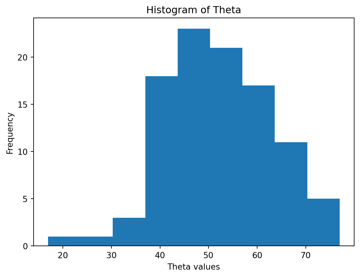
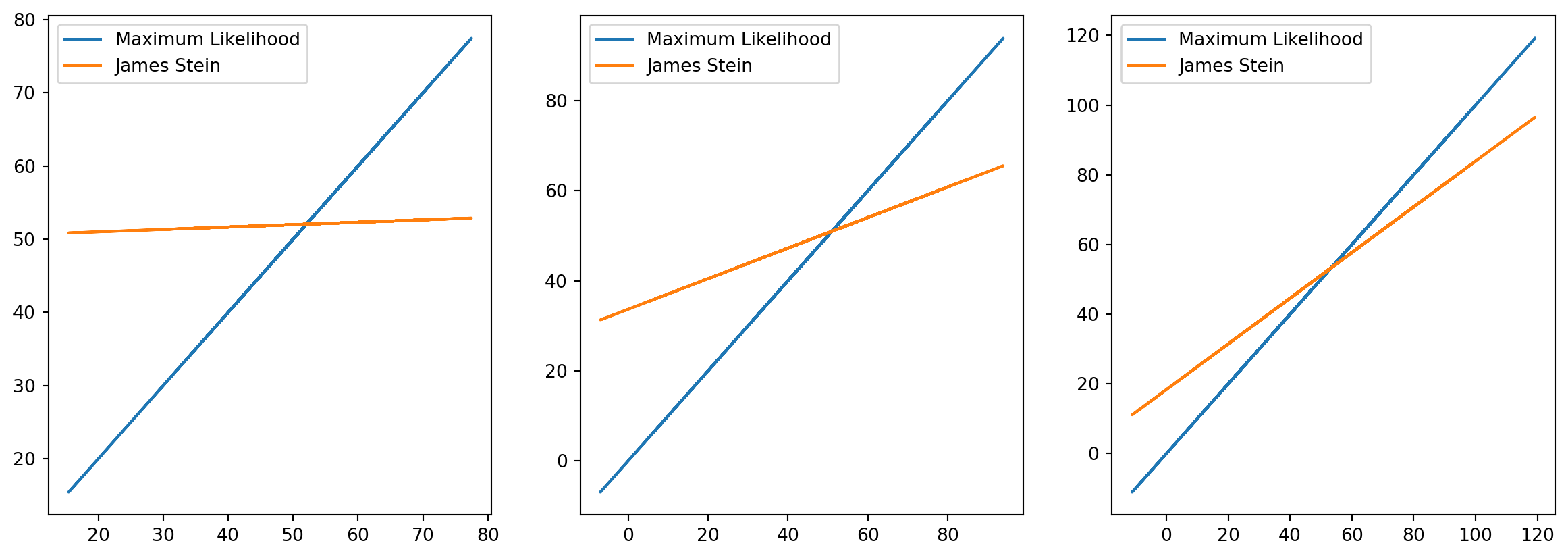
To illustrate the idea, we will show an example of how we can implement the positive part JS estimator and show that it improves the mean square error between the estimated value and the true value compared to the maximum likelihood estimate. We will assume that the true friction measurements on the 100 sections have mean 50 and standard deviation of 10. For the device we are using to measure the friction, the standard deviation of the measurement is know and we will look at three cases where the standard deviation is 2, 10, and 30. We will compared the mean square error of the JS estimator and the maximum likelihood estimator.

import numpy as np
import matplotlib.pyplot as plt

# Function to calculate James-Stein Estimator
def james_stein(x, error_std):
    n = len(x)
    variance = error_std**2
    theta_hat = ((n - 3) * variance / np.sum((x - np.mean(x))**2)) * x + ((1 - (n - 3) * variance / np.sum((x - np.mean(x))**2)) * np.mean(x))
    return theta_hat

# Generating normally distributed true friction values
theta = 50 + 10 * np.random.randn(100)
plt.hist(theta, bins='auto')  # 'bins' can be set to an integer for a specific number of bins or 'auto' for automatic binning
plt.title('Histogram of Theta')
plt.xlabel('Theta values')
plt.ylabel('Frequency')
plt.show()

# Measurements with different measurement error standard deviations
x2 = theta + 2 * np.random.randn(100)
x10 = theta + 10 * np.random.randn(100)
x20 = theta + 20 * np.random.randn(100)

# Calculating James-Stein estimator for each case
theta_hat2 = james_stein(x2, 2)
theta_hat10 = james_stein(x10, 10)
theta_hat20 = james_stein(x20, 20)

# Calculating MSE
MSE = np.array([
    [np.mean((theta - x2)**2), np.mean((theta - theta_hat2)**2)],
    [np.mean((theta - x10)**2), np.mean((theta - theta_hat10)**2)],
    [np.mean((theta - x20)**2), np.mean((theta - theta_hat20)**2)]
])

print("MSE:")
print(MSE)

MSE:
[[  4.07847652 110.69315578]
 [121.19202847  56.00276867]
 [504.79429861 238.55737768]]

# Plotting
plt.figure(figsize=(15, 5))

plt.subplot(1, 3, 1)
plt.plot(x2, x2, label='Maximum Likelihood')
plt.plot(x2, theta_hat2, label='James Stein')
plt.legend()

plt.subplot(1, 3, 2)
plt.plot(x10, x10, label='Maximum Likelihood')
plt.plot(x10, theta_hat10, label='James Stein')
plt.legend()

plt.subplot(1, 3, 3)
plt.plot(x20, x20, label='Maximum Likelihood')
plt.plot(x20, theta_hat20, label='James Stein')
plt.legend()

plt.show()

The figure shows how the the James-Stein estimator shrinks the measurement towards the average of the measurements (here 50). For the case where the measurement error is very small, the measurements are almost unchanged by the JS estimator. As the measurement error increases, more weight is placed on the average and the amount of shrinkage is more pronounced.