Cardiotocograms (CTGs) and fetal health

The reduction of child mortality, a central objective in several of the United Nations’ Sustainable Development Goals, stands as a crucial measure of human progress. In this context, Cardiotocograms (CTGs) emerge as an effective and economically viable method to monitor fetal health. They equip healthcare professionals with vital data, enabling timely interventions to prevent both child and maternal mortality. Functioning through the emission and reception of ultrasound pulses, CTGs provide critical insights into fetal heart rate (FHR), fetal movements, uterine contractions, and other significant parameters, thereby playing a pivotal role in prenatal care.

In clinical environments, specialized procedures exist to evaluate whether a patient’s Cardiotocogram (CTG) is normal, a process that necessitates expert domain knowledge. As machine learning technology advances, there is growing potential to develop sophisticated models that can classify fetal health more efficiently. These models would be based on features extracted from CTG outputs, aiming to enhance the prediction of child and maternal mortality. This integration of machine learning into fetal health assessment represents a significant stride towards more accurate and accessible prenatal care.

Dataset and Model description

In this blog, we explore the use of a Kaggle dataset to classify fetal health conditions using machine learning models. This dataset comprises 2126 instances of features derived from Cardiotocogram (CTG) exams. These features have been categorized into three classes by expert obstetricians: Normal, Suspect, and Pathological. Our objective is to develop a multiclass model capable of accurately classifying CTG features into these three distinct fetal health states, demonstrating the potential of machine learning in enhancing prenatal care diagnostics.

Here are steps of implementing the machine learning models to do the classification:

Load & Pre-process data: Handling missing values, outliers, etc.
Label encoding: Split data into training dataset and test dataset, and transform data by scaling and normalization, which makes continuous variables into a common scale to ease the comparison between variables with various units and ranges.
Modeling
Evaluation

Step 1: Load & Pre-process data

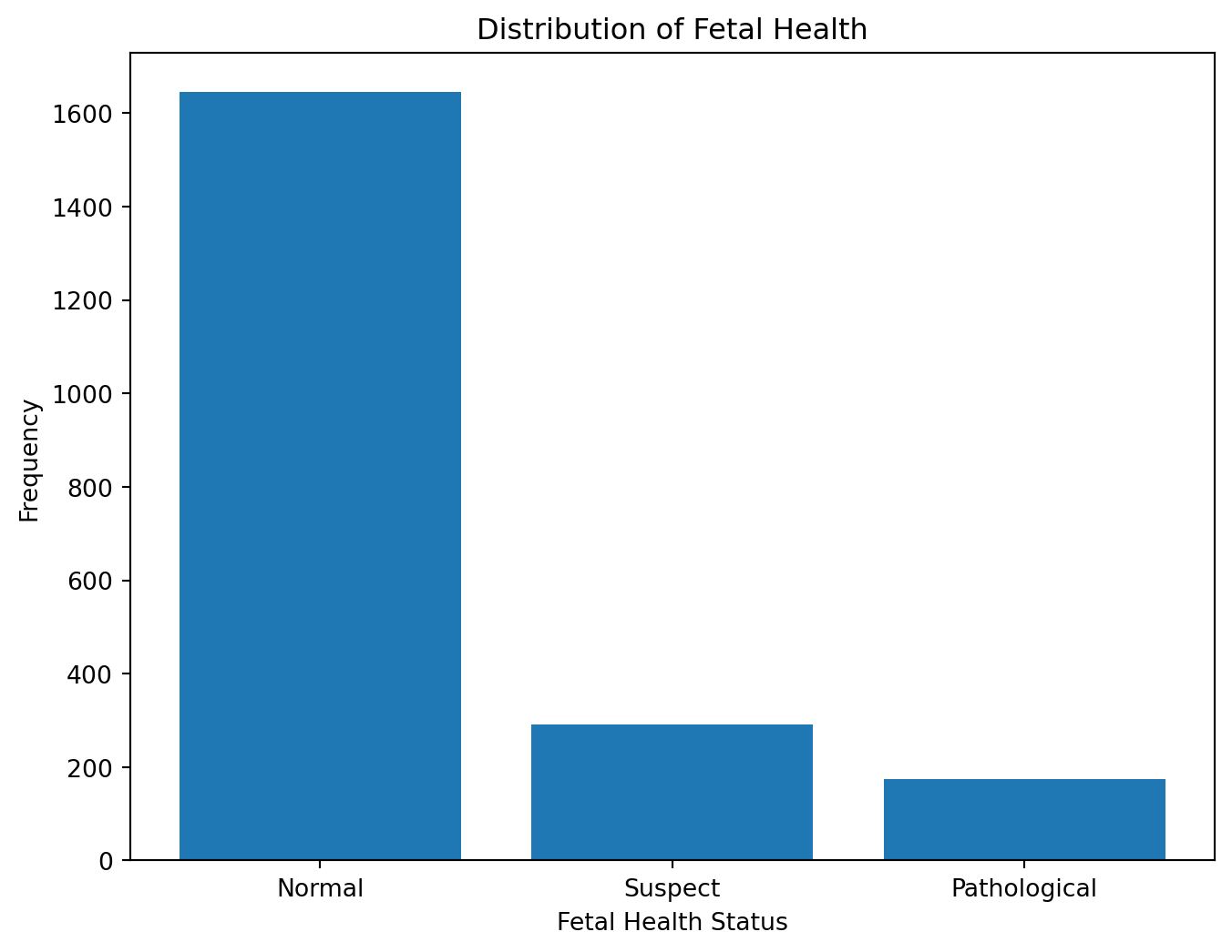
The histogram below provides a visual overview of how the fetal health cases are distributed across these three categories, indicating the relative frequencies of normal, suspect, and pathological fetal health conditions in the dataset.

# import library
import numpy as np 
import pandas as pd
from scipy import stats
from sklearn import preprocessing
import matplotlib.pyplot as plt
import seaborn as sns
from sklearn.impute import KNNImputer
from sklearn.preprocessing import MinMaxScaler
from sklearn.naive_bayes import MultinomialNB
from sklearn.linear_model import LogisticRegression
from sklearn.tree import DecisionTreeClassifier
from sklearn.ensemble import RandomForestClassifier
from sklearn.neighbors import KNeighborsClassifier
from sklearn.svm import SVC
from sklearn.ensemble import GradientBoostingClassifier
from sklearn.model_selection import train_test_split
from sklearn.metrics import confusion_matrix, accuracy_score, precision_score, recall_score, f1_score
# load & preprocess data
df = pd.read_csv('https://raw.githubusercontent.com/xiaoyingyang96/xiaoyingyang96.github.io/main/Data/fetal_health.csv')

#handle missing values, drop duplicated row
df.isnull().sum()
df = df.drop_duplicates()

# Plotting the histogram for the distribution of fetal_health
plt.figure(figsize=(8, 6))
plt.hist(df['fetal_health'], bins=np.arange(1, 5) - 0.5, rwidth=0.8)
plt.xticks(ticks=[1, 2, 3], labels=['Normal', 'Suspect', 'Pathological'])
plt.xlabel('Fetal Health Status')
plt.ylabel('Frequency')
plt.title('Distribution of Fetal Health')
plt.show()

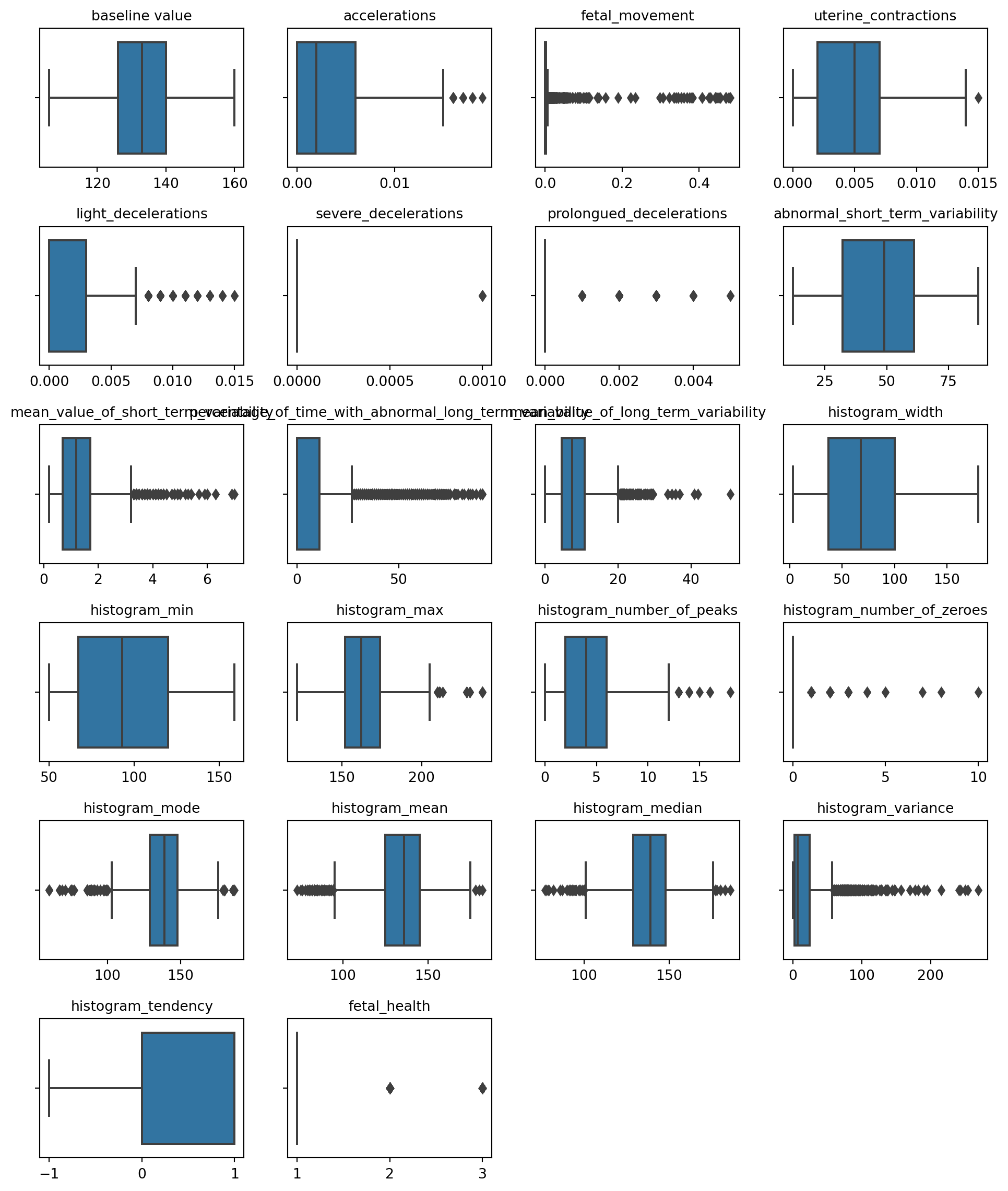
# Handling outlier for numeric attributes 
# Create a 2x3 grid of subplots
fig, axes = plt.subplots(6, 4, figsize=(10, 12))
axes = axes.flatten()
    
# Create a boxplot for each continuous variable
for i, column in enumerate(df.columns):
    sns.boxplot(data=df, x=column, ax=axes[i])
    axes[i].set_title(f"{column}", fontsize=10)
    axes[i].set_xlabel("")  # Remove x-axis title

# Remove empty subplot
for i in range(len(df.columns), len(axes)):
    fig.delaxes(axes[i])

# Adjust layout
plt.tight_layout()
plt.show()

Boxplots are useful for indicating whether a distribution is skewed and whether there are potential unusual observations (outliers) in the dataset. In this example we applied boxplots to explore outliers from each data and diagrams for each attribute are presented above. The boxplots reveal outliers in several attributes. Nonetheless, considering that the dataset has been reviewed and interpreted by clinic experts, the apparent outliers identified in the boxplots might not be anomalous in a clinical setting. Rather, they may signify clinically relevant variations, such as indicators of fetal distress or maternal health conditions. No action will be taken on these values that out of boxplot range.

Step 2: Label encoding

The dataset was split into 2 parts. 30% of the data will be reserved for testing, and 70% will be used for training. Then the “fit-transform” method is called on the scaler object to scale the training data. This method computes the minimum and maximum values to be used for later scaling(fit), and then scales the training data(transform).

#Label encoding
#Dara Splitting
df_features = df.drop(['fetal_health'], axis=1)
df_target = df['fetal_health']

# split df at 70-30 ratio
X_train, X_test, y_train, y_test = train_test_split(df_features, df_target, test_size=0.3, random_state=123)

# Initialize the MinMaxScaler object
scaler = MinMaxScaler()

# Fit the scaler on the training data and transform the training data
scaled_X_train = scaler.fit_transform(X_train)
# Transform the test data using the fitted scaler
scaled_X_test = scaler.transform(X_test)  # Only transform, no fitting

#Convert the scaled training data back to a DataFrame
scaled_X_train = pd.DataFrame(scaled_X_train, columns = X_train.columns, index=X_train.index)
scaled_X_train.head()

	baseline value	accelerations	fetal_movement	uterine_contractions	light_decelerations	abnormal_short_term_variability	mean_value_of_short_term_variability	percentage_of_time_with_abnormal_long_term_variability	...	histogram_width	histogram_min	histogram_max	histogram_number_of_peaks	histogram_number_of_zeroes	histogram_mode	histogram_mean	histogram_median	histogram_variance	histogram_tendency
468	0.703704	0.000000	0.004158	0.133333	0.000000	0.960000	0.014706	0.373626	...	0.197740	0.759259	0.413793	0.111111	0.0	0.666667	0.642202	0.620370	0.000000	0.0
1143	0.296296	0.222222	0.000000	0.400000	0.400000	0.120000	0.220588	0.000000	...	0.372881	0.222222	0.181034	0.222222	0.0	0.579365	0.440367	0.444444	0.118959	1.0
162	0.296296	0.222222	0.000000	0.400000	0.066667	0.266667	0.147059	0.109890	...	0.440678	0.157407	0.224138	0.111111	0.0	0.515873	0.467890	0.444444	0.029740	1.0
919	0.296296	0.000000	0.000000	0.266667	0.000000	0.360000	0.088235	0.109890	...	0.112994	0.518519	0.060345	0.055556	0.0	0.500000	0.422018	0.398148	0.007435	0.5
1103	0.296296	0.388889	0.000000	0.200000	0.000000	0.093333	0.308824	0.000000	...	0.282486	0.500000	0.301724	0.111111	0.1	0.515873	0.495413	0.462963	0.029740	0.5

5 rows × 21 columns

In machine learning, we CANNOT “fit” the scaler to the test data because doing so would make the model indirectly aware of the specifics of the test data. If we fit on the test data, the scaler will adjust its parameters according to the range of the test data, which is equivalent to leaking information about the test data during the training phase of the model. This can lead to overfitting the model to the test data, which affects our purpose of realistically evaluating the generalization ability of the model.
The correct approach is to only fit on the training data and use this fitted scaler to transform the test data. This ensures that our model evaluation is fair because the test data is scaled to the range of the training data, not its own range. In short, this ensures that the data in the test phase is not previously seen by the model, thus providing a fair assessment of the model’s performance when dealing with new data. The test data fitted by scaler from training data is shown as below.

scaled_X_test = pd.DataFrame(scaled_X_test, columns = X_test.columns, index=X_test.index)
scaled_X_test.head()

	baseline value	accelerations	fetal_movement	uterine_contractions	abnormal_short_term_variability	mean_value_of_short_term_variability	percentage_of_time_with_abnormal_long_term_variability	...	histogram_width	histogram_min	histogram_max	histogram_number_of_peaks	histogram_mode	histogram_mean	histogram_median	histogram_variance	histogram_tendency
1542	0.703704	0.166667	0.000000	0.533333	0.480000	0.073529	0.065934	...	0.248588	0.648148	0.387931	0.166667	0.698413	0.697248	0.666667	0.011152	0.5
753	0.444444	0.000000	0.002079	0.000000	0.586667	0.044118	0.362637	...	0.090395	0.694444	0.189655	0.111111	0.547619	0.532110	0.500000	0.007435	0.0
454	0.500000	0.000000	0.006237	0.200000	0.613333	0.044118	0.186813	...	0.107345	0.694444	0.215517	0.111111	0.603175	0.577982	0.546296	0.003717	0.5
534	0.574074	0.000000	0.000000	0.000000	0.680000	0.044118	0.395604	...	0.525424	0.194444	0.387931	0.166667	0.658730	0.623853	0.601852	0.003717	1.0
599	0.777778	0.000000	0.008316	0.266667	0.840000	0.058824	0.000000	...	0.163842	0.833333	0.431034	0.055556	0.714286	0.706422	0.675926	0.000000	0.0

5 rows × 21 columns

Step 3: Modeling

In this study, Machine Learning algorithms including Naive Bayes, Logistic Regression, Decision Tree, Random Forest, K-Nearest Neighbors (KNN), and Support Vector Machines (SVM) are applied to train models.

Model 1: Naive Bayes

# Naive Bayes
naive_bayes = MultinomialNB()

# Train the NB model on the train data
naive_bayes.fit(scaled_X_train, y_train)

# Predict on test data
y_pred_nb = naive_bayes.predict(scaled_X_test)

# Calculate evaluation metrics
accuracy_nb = accuracy_score(y_test, y_pred_nb)
precision_nb = precision_score(y_test, y_pred_nb, average='weighted')
recall_nb = recall_score(y_test, y_pred_nb, average='weighted')
f1_nb = f1_score(y_test, y_pred_nb, average='weighted')

# Print results
print("Accuracy:", round(accuracy_nb, 3))
print("Precision:", round(precision_nb, 3))
print("Recall:", round(recall_nb, 3))
print("F1-Score:", round(f1_nb, 3))

Accuracy: 0.809
Precision: 0.792
Recall: 0.809
F1-Score: 0.75

Model 2: Logistic Regression

# Logistic regression 
log_reg = LogisticRegression(random_state=123)

# Train the LR model on the train data
log_reg.fit(scaled_X_train, y_train)

# Predict on test data
y_pred_lr = log_reg.predict(scaled_X_test)

# Calculate evaluation metrics
accuracy_lr = accuracy_score(y_test, y_pred_lr)
precision_lr = precision_score(y_test, y_pred_lr, average='weighted')
recall_lr = recall_score(y_test, y_pred_lr, average='weighted')
f1_lr = f1_score(y_test, y_pred_lr, average='weighted')

# Print results
print("Accuracy:", round(accuracy_lr, 3))
print("Precision:", round(precision_lr, 3))
print("Recall:", round(recall_lr, 3))
print("F1-Score:", round(f1_lr, 3))

Accuracy: 0.901
Precision: 0.896
Recall: 0.901
F1-Score: 0.897

Model 3: Decision Tree

# Decision tree 
d_tree = DecisionTreeClassifier(random_state=123)

# Train the DT model on the train data
d_tree.fit(scaled_X_train, y_train)

# Predict on test data
y_pred_dt = d_tree.predict(scaled_X_test)

# Calculate evaluation metrics
accuracy_dt = accuracy_score(y_test, y_pred_dt)
precision_dt = precision_score(y_test, y_pred_dt, average='weighted')
recall_dt = recall_score(y_test, y_pred_dt, average='weighted')
f1_dt = f1_score(y_test, y_pred_dt, average='weighted')

# Print results
print("Accuracy:", round(accuracy_dt, 3))
print("Precision:", round(precision_dt, 3))
print("Recall:", round(recall_dt, 3))
print("F1-Score:", round(f1_dt, 3))

Accuracy: 0.92
Precision: 0.923
Recall: 0.92
F1-Score: 0.921

Model 4: Random Forest

# Random forest
r_forest = RandomForestClassifier(random_state=123)

# Train the DT model on the train data
r_forest.fit(scaled_X_train, y_train)

# Predict on test data
y_pred_rf = r_forest.predict(scaled_X_test)

# Calculate evaluation metrics
accuracy_rf = accuracy_score(y_test, y_pred_rf)
precision_rf = precision_score(y_test, y_pred_rf, average='weighted')
recall_rf = recall_score(y_test, y_pred_rf, average='weighted')
f1_rf = f1_score(y_test, y_pred_rf, average='weighted')

# Print results
print("Accuracy:", round(accuracy_rf, 3))
print("Precision:", round(precision_rf, 3))
print("Recall:", round(recall_rf, 3))
print("F1-Score:", round(f1_rf, 3))

Accuracy: 0.946
Precision: 0.946
Recall: 0.946
F1-Score: 0.946

Model 5: K-Nearest Neighbors (KNN)

import numpy as np
from sklearn.neighbors import KNeighborsClassifier
from sklearn.metrics import accuracy_score, precision_score, recall_score, f1_score

# Ensure that scaled_X_train and scaled_X_test are C-ordered NumPy arrays
scaled_X_train = np.ascontiguousarray(scaled_X_train)
scaled_X_test = np.ascontiguousarray(scaled_X_test)

# Initialization and training of KNN classifiers
knn = KNeighborsClassifier()
knn.fit(scaled_X_train, y_train)

# Predictions on the test set
y_pred_knn = knn.predict(scaled_X_test)

# Calculation of evaluation indicators
accuracy_knn = accuracy_score(y_test, y_pred_knn)
precision_knn = precision_score(y_test, y_pred_knn, average='weighted')
recall_knn = recall_score(y_test, y_pred_knn, average='weighted')
f1_knn = f1_score(y_test, y_pred_knn, average='weighted')

# 打印结果
print("Accuracy:", round(accuracy_knn, 3))
print("Precision:", round(precision_knn, 3))
print("Recall:", round(recall_knn, 3))
print("F1-Score:", round(f1_knn, 3))

Accuracy: 0.907
Precision: 0.903
Recall: 0.907
F1-Score: 0.901

Model 6: Support Vector Machines (SVM)

# Support vector machines classifier 
svm = SVC(random_state=123)

# Train SVC on train data
svm.fit(scaled_X_train, y_train)

# Predict on the test data
y_pred_svm = svm.predict(scaled_X_test)

# Calculate evaluation metrics
accuracy_svm = accuracy_score(y_test, y_pred_svm)
precision_svm = precision_score(y_test, y_pred_svm, average='weighted')
recall_svm = recall_score(y_test, y_pred_svm, average='weighted')
f1_svm = f1_score(y_test, y_pred_svm, average='weighted')

# Print results
print("Accuracy:", round(accuracy_svm, 3))
print("Precision:", round(precision_svm, 3))
print("Recall:", round(recall_svm, 3))
print("F1-Score:", round(f1_svm, 3))

Accuracy: 0.913
Precision: 0.912
Recall: 0.913
F1-Score: 0.911

Step 5: Evaluation

The performance of each machine learning model, trained using various algorithms, is evaluated using metrics such as accuracy, precision, recall, and F1-Score. These metrics provide a comprehensive understanding of different facets of model performance, enabling the selection of the most effective model. Metrics have shown in belowing table. As a result, the model trained by random forest algorithm has the best performance among 6 models.

Model No.	ML Algorithm	Accuracy	Precision	Recall	F1-Score
1	Naive Bayes	0.809	0.792	0.809	0.75
2	Logistic Regression	0.901	0.896	0.901	0.897
3	Decision Tree	0.92	0.923	0.92	0.921
4	Random Forest	0.946	0.946	0.946	0.946
5	KNN	0.907	0.903	0.907	0.901
6	SVM	0.913	0.912	0.913	0.911

Reference